How to Use TODAY() to Highlight Fast-Approaching Dates in an Excel Sheet

Use Microsoft Excel’s TODAY() function in simple expressions to highlight the current date and past and future dates.

Many applications track dates for lots of different reasons. You might track due dates, delivery dates, appointments and so on. Depending how you use these dates, you might want to highlight specific dates as they approach the current date in Microsoft Excel. Similarly, you might want to highlight future dates.

Using the TODAY() function and a few conditional highlighting rules, you’ll never get caught unaware.

Jump to:

Highlight today in Microsoft Excel

While you probably won’t want to wait until a due date to start a project, highlighting the current date can help alert you when timing is essential. Fortunately, Excel’s TODAY() function always equals the current date, so you don’t have to update the rule or even include an input value.

SEE: Explore these 87 Excel tips every user should master.

Let’s add a conditional format that always highlights the current date:

1. Select the cells or rows you want to highlight. In this case, select B3:E12 — the data range.
2. Click the Home tab, and then, click Conditional Formatting in the Styles group and choose Highlight Cells Rules.
3. Choose A Date Occurring.
4. In the resulting dialog, choose Today from the first dropdown, and then, choose Light Red Fill from the second (Figure A). As you can see, the current date is December 6.

Figure A

5. Click OK.

This method is the easiest way to quickly apply a conditional format to highlight the current date, but it is a bit limited. First, you have only a few format combinations available. Second, it doesn’t highlight the entire row — only the cell containing the date. This rule is able to detect dates in the selected range and apply the format only to those cells. So, it doesn’t matter where the date column is in relation to the selected range.

SEE: Check out these ways to suppress 0 in Excel.

Highlight yesterday in Microsoft Excel

There are built-in rules for yesterday and tomorrow, but let’s enter a rule instead, so you’ll know how to do so when there isn’t an adequate built-in rule. Let’s start with yesterday:

1. Select the data range B3:E12.
2. Click the Home tab. Then, click Conditional Formatting in the Styles group, and choose New Rule.
3. In the resulting dialog, select the Use a Formula to Determine Which Cells To Format option in the top pane.
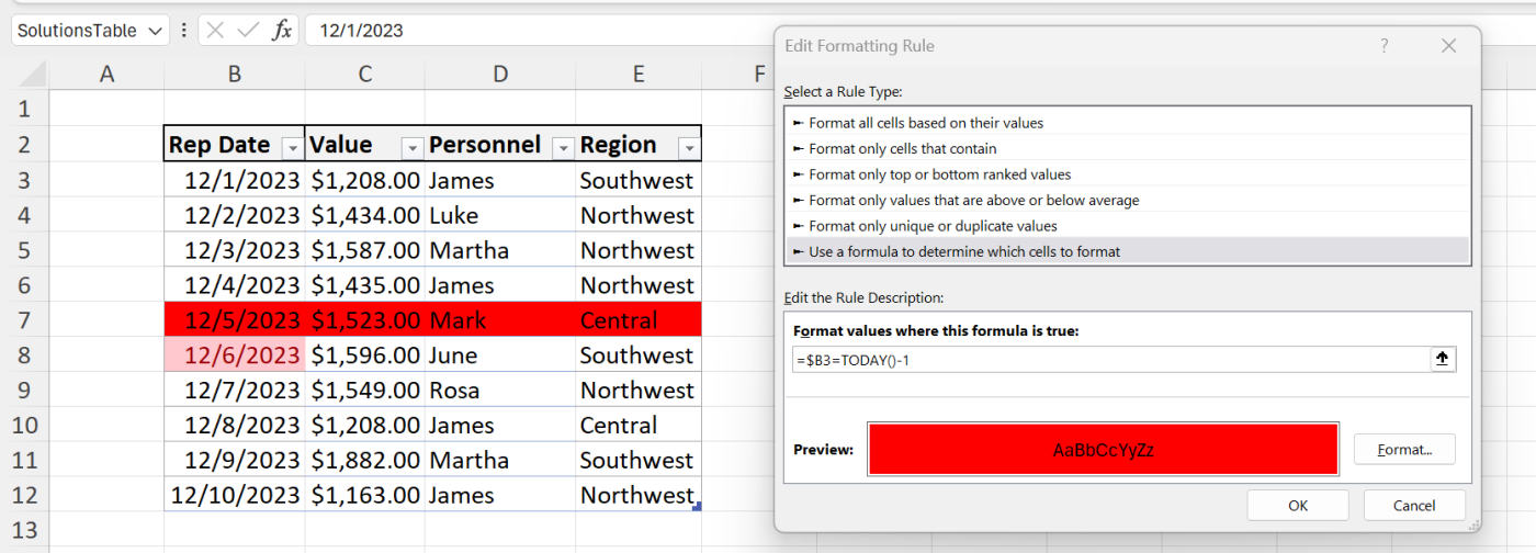
4. In the bottom pane, enter the expression =$B3=TODAY()-1. The simple expression TODAY()-1 subtracts one from the current date. That’s the same thing as yesterday.
5. Click Format.
6. Click the Fill tab, choose red and click OK. Figure B shows the rule and the format.

Figure B

7. Click OK to apply the format.

As you can see in Figure B, the rule highlights the entire record when the date in column B is yesterday. Notice that the rule has an absolute column reference ($B). If you omit the dollar sign, Excel applies the highlight to the cell instead of the entire row. The reference to row 3 isn’t absolute, so the rule can evaluate all of the rows in the selected range.

SEE: Here’s how to parse data in Microsoft Excel.

Highlight tomorrow in Microsoft Excel

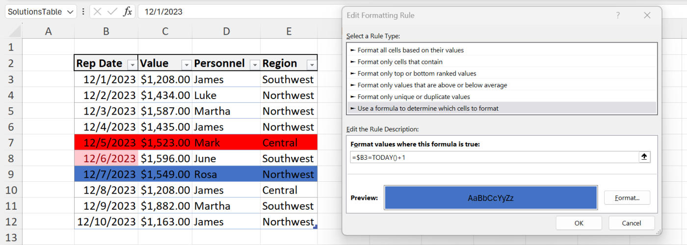
To highlight tomorrow, repeat the above steps, but enter the rule =$B3=TODAY()+1, as shown in Figure C. Click Format, and choose any color, but I chose medium blue. Click OK (twice) to apply the format, which highlights the entire row when the date in column B is tomorrow. Again, the absolute and relative referencing is important.

Figure C

All three rules are simple to implement, but they are limited to today, yesterday and tomorrow. What if you want to highlight other daily increments beyond these three?

Highlight past dates in Microsoft Excel

There may come a time when you’ll want a bit more flexibility when highlighting important dates. For instance, you might want to highlight dates that are a week ahead or a week past. When this is the case, I recommend using an input cell where you can specify the number of days. By referencing the input cell in the formula, the highlight will update automatically depending on your needs at the time.

Using Figure D as a guide, format two input cells: days in the past and days into the future. Accordingly, we’ll reference C1 in the past rule and C2 in the future.

Figure D

First, let’s enter the rule for the past:

1. Select the data range B5:E14. Notice that I’ve updated the range rows because I inserted rows for the input cells.
2. Click the Home tab. Then, click Conditional Formatting in the Styles group, and choose New Rule.
3. In the resulting dialog, select the Use a Formula to Determine Which Cells To Format option in the top pane.
4. In the bottom pane, enter the expression =$B5=TODAY()-$C$1.
5. Click Format.
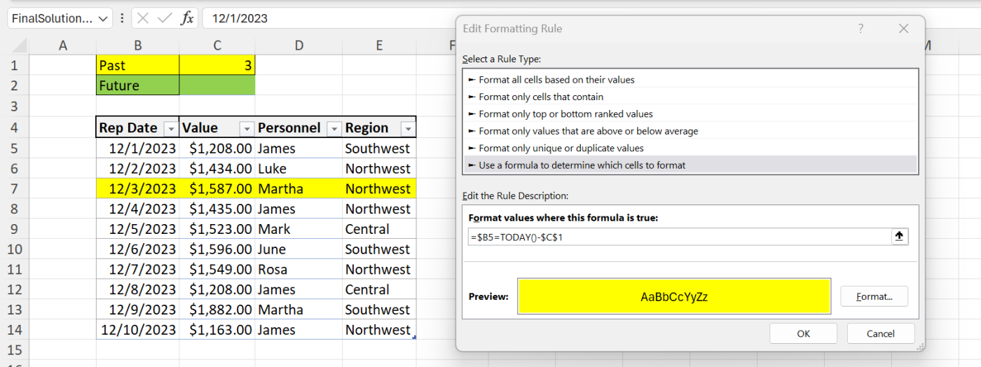
6. Click the Fill tab, choose yellow and click OK. Figure E shows the rule and the format.

Figure E

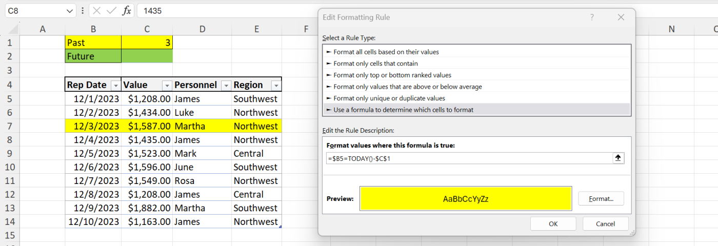
7. Click OK to apply the format.

Figure E shows the result of entering 3 in C. Once again, the absolute address, $C$1 is important. If you leave this relative, the highlight won’t work as expected. When C1 is empty or contains 0, this rule highlights the current day.

SEE: Discover how to adjust text to fit in Excel cells.

Highlight future dates in Microsoft Excel

Repeat the steps above to apply a highlight for the future. Except in step 4, enter the expression =$B5=TODAY()+$C$2, and choose green. Figure F shows the resulting sheet after entering the value 3 into C2.

Figure F

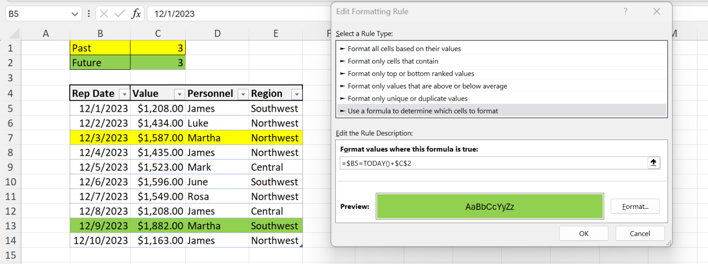
With the input cells and rules in place, feel free to change the values in C1 and C2. If the value is too far into the past or into the future for the existing dates, Excel won’t apply the highlight. Go ahead now and change those dates to see how both rules work.

Helpful hints

When applying conditional formats, the position of the rule is important. The last rules you enter will take precedence because they’re the first Excel evaluates. When several rules are in play, Excel might not apply them in the order you expect.

To change this, open the rules using Manage Rules on the Conditional Formatting dropdown and move the rules accordingly. One more thing that you might consider. Use the fill color of C1 and C2 to match the highlight fill color in the rule, as shown in Figures E and F. Doing so will offer a visual clue for the users, so they don’t have to remember what those two colors mean.